5 more Excel VBA toolbar shortcuts that work in every spreadsheet I open

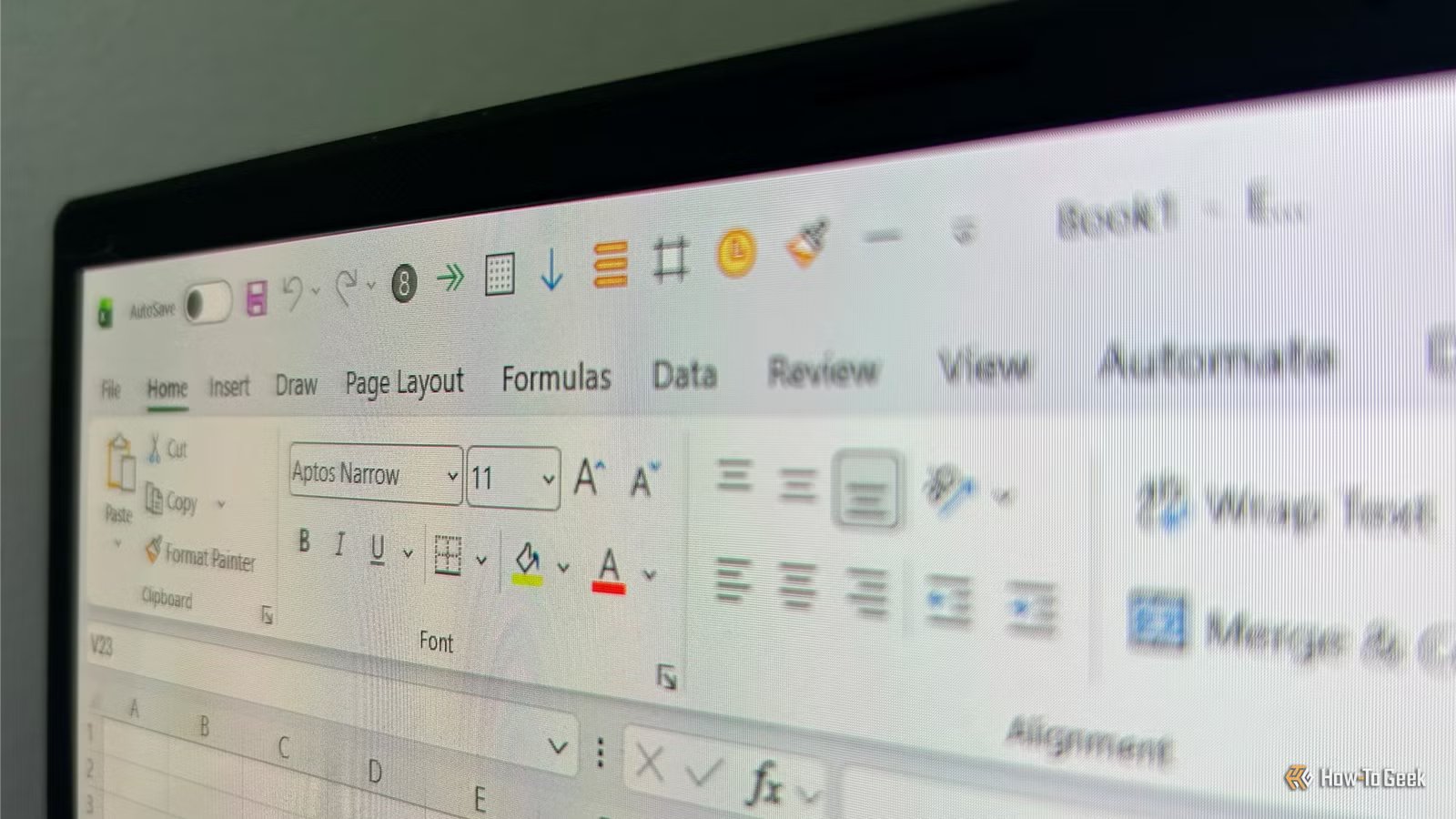
The first VBA macros I added to my Excel toolbar quickly became some of my most-used shortcuts. Since then, I’ve added five more that save me even more time by automating repetitive formatting, cleanup, and navigation tasks in every workbook I open.

Access your Personal Macro Workbook

Find the right place for your new code

The Personal Macro Workbook (PERSONAL.XLSB) is a hidden file that loads every time Excel starts, making your macros available in every workbook you open.

If this is your first time creating personal macros, you need to generate the workbook before adding these tools:

1. Open a blank Excel workbook and go to the View tab.
2. Click the Macros drop-down arrow, then select Record Macro.
3. In the Store macro in drop-down menu, select Personal Macro Workbook, then click OK.
4. Click the square Stop Recording button in the bottom-left corner of the Excel window. Excel creates PERSONAL.XLSB automatically, ready for your VBA code.
5. Press Alt+F11 or click Developer > Visual Basic to open the VBA Editor, right-click VBAProject (PERSONAL.XLSB), choose Insert > Module, and open the new module.

If you already created a Personal Macro Workbook, open it directly:

1. Press Alt+F11 or click Developer > Visual Basic.
2. In the Project Explorer pane, find and expand VBAProject (PERSONAL.XLSB) in the folder tree.
3. Open the Modules folder nested beneath the project name.
4. Double-click the module containing your existing macros to display the code workspace on the right side.

OS

Windows, macOS, iPhone, iPad, Android

Free trial

1 month

Microsoft 365 includes access to Office apps like Word, Excel, and PowerPoint on up to five devices, 1 TB of OneDrive storage, and more.

Add the new macros

Keep each macro as a separate procedure

You can add as many or as few of these macros as you like. Paste the ones you choose into the same module, making sure each procedure starts with its own Sub statement and ends with its own End Sub statement.

When you’ve finished, the module will look something like this, with any existing macros at the top and these new ones beneath:

Paste values and formats in one click

Excel has separate options for pasting values and formatting, but it doesn’t let you combine them in a single action. This macro combines the two, preserving the formatting while pasting only the calculated values rather than the original formulas.

Sub PasteValuesAndFormats()
    Selection.PasteSpecial Paste:=xlPasteValues
    Selection.PasteSpecial Paste:=xlPasteFormats
End Sub

Delete only completely blank rows

Excel’s Go To Special > Blanks workflow can remove rows containing any blank cells, making it risky for datasets with optional fields. This macro removes only rows that are completely empty.

Sub DeleteEntirelyBlankRows()
    Dim LastRow As Long
    Dim i As Long
    
    LastRow = ActiveSheet.UsedRange.Rows.Count + ActiveSheet.UsedRange.Row - 1
    
    Application.ScreenUpdating = False
    For i = LastRow To 1 Step -1
        If WorksheetFunction.CountA(ActiveSheet.Rows(i)) = 0 Then
            ActiveSheet.Rows(i).Delete
        End If
    Next i
    Application.ScreenUpdating = True
End Sub

Generate a clickable sheet index

Navigating large workbooks with dozens of tabs is tedious. This macro creates a clickable table of contents on a dedicated sheet, and when worksheets are added, renamed, or deleted, running it again rebuilds the index, replacing any previous Sheet Index.

Sub CreateHyperlinkedIndex()
    Dim ws As Worksheet
    Dim indexSheet As Worksheet
    Dim i As Long
    
    On Error Resume Next
    Application.DisplayAlerts = False
    ActiveWorkbook.Sheets("Sheet Index").Delete
    Application.DisplayAlerts = True
    On Error GoTo 0
    
    Set indexSheet = ActiveWorkbook.Sheets.Add(Before:=ActiveWorkbook.Sheets(1))
    indexSheet.Name = "Sheet Index"
    indexSheet.Cells(1, 1).Value = "Workbook Index (Click to Navigate)"
    indexSheet.Cells(1, 1).Font.Bold = True
    
    i = 3
    For Each ws In ActiveWorkbook.Worksheets
        If ws.Name <> indexSheet.Name Then
            indexSheet.Hyperlinks.Add _
                Anchor:=indexSheet.Cells(i, 1), _
                Address:="", _
                SubAddress:="'" & ws.Name & "'!A1", _
                TextToDisplay:=ws.Name
            i = i + 1
        End If
    Next ws
    
    indexSheet.Columns(1).AutoFit
End Sub

Insert a static date and time

The default NOW() function updates every time your spreadsheet recalculates, which ruins its use as a historical record. This snippet inserts a hard-coded date and time stamp that remains permanently frozen on the exact second you clicked the button.

Sub InsertStaticDateTime()
    ActiveCell.Value = Now
    ActiveCell.NumberFormat = "yyyy-mm-dd hh:mm:ss"
End Sub

Jump to your data’s bottom-right corner

Unlike Excel’s built-in navigation shortcuts, this macro ignores “ghost cells” caused by old formatting and jumps to the intersection of your last row and last column containing data. If your data reaches column S and row 29, for example, it takes you straight to S29.

Sub GoToDataCorner()
    Dim RealLastRow As Long
    Dim RealLastCol As Long
    
    On Error Resume Next
    RealLastRow = Cells.Find("*", SearchOrder:=xlByRows, SearchDirection:=xlPrevious).Row
    RealLastCol = Cells.Find("*", SearchOrder:=xlByColumns, SearchDirection:=xlPrevious).Column
    On Error GoTo 0
    
    If RealLastRow = 0 Then RealLastRow = 1
    If RealLastCol = 0 Then RealLastCol = 1
    
    Cells(RealLastRow, RealLastCol).Select
End Sub

Add your new macros to the QAT

Run your shortcuts with a single click

Whether these are your first macros or you’re adding to an existing collection, the process is the same.

To open the QAT settings:

1. Right-click anywhere on the Excel ribbon and select Show Quick Access Toolbar if that option appears. If it doesn’t, your QAT is already visible.
2. Click the small drop-down arrow on the right side of the toolbar, then click More Commands.
3. In the Choose commands from drop-down menu, select Macros.
4. Select each of your new macros from the left column and click Add to move them to the toolbar list. Any macros you’ve already added to your QAT will also be listed there.
5. Select the added macro in the right column, click Modify, and choose an icon that makes it easy to identify.

When exiting Excel, you may see a prompt asking if you want to save changes made to the Personal Macro Workbook. Always click Save. If you skip this step, your new macros will disappear the next time you open the app.

Build Excel around the way you work

By building your own tools in Excel, you can create a faster, more personalized workflow that matches the way you actually use spreadsheets. But macros aren’t the only way to customize Excel to fit your habits. You can also make everyday tasks smoother by creating a custom tab on the ribbon, building tailored autofill options with custom lists, and giving your PivotTables a more polished look by changing slicer styles.