A multi-agent system for automating scientific discovery

Robin implementation

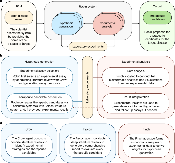
Robin was implemented as a Jupyter notebook using the Aviary framework to instantiate and call agents³³. Robin utilizes the OpenAI o4-mini model to synthesize literature and generate hypotheses, and the Anthropic Claude 3.7 Sonnet model as the judge for pairwise comparisons to rank hypotheses. Prompts used for agents and LLMs called in Robin are shown in Supplementary Figs. 2–11.

Of note, although the experiments in this paper were conducted using an agentic implementation of Robin, we observed that Robin almost always called tools in the same order, leading to a deterministic workflow. Therefore, we translated Robin into a streamlined Jupyter notebook to improve stability and ease of use.

The ranking of hypotheses was calculated via a series of pairwise comparisons adjudicated by the LLM judge. When ranking 25 or fewer hypotheses, all possible pairs were compared in a round robin tournament. When considering more than 25 hypotheses, 300 pairwise comparisons were randomly selected to achieve a comprehensive assessment within reasonable computational and time constraints. The outcomes from these comparisons were used to estimate strength parameters via the Bradley–Terry–Luce (BTL) model, which subsequently informed the relative ranking of each hypothesis⁵⁴. Although there is no clear consensus on the optimal strategy for LLM-judge-based rankings, we opted for pairwise comparisons rather than pointwise. Some literature^55,56 has shown pairwise comparisons to be more robust than pointwise grading, as pointwise grading may be unable to distinguish nuanced differences between similar pairs. Position bias in the pairwise comparisons is addressed by utilizing a highly distributed tournament paired with the BTL model, rather than relying on simple win–loss tallies, which are highly susceptible to positional bias. To generate the prompt for this LLM judge, domain experts were asked to conduct pairwise comparisons of the therapeutic candidate hypotheses in Robin. The results of these expert evaluations were given to Google’s Gemini 2.5 Pro Preview model to generate a prompt for the LLM judge in Robin. This approach was designed to elicit decision-making from the LLM judge consistent with expert preferences and criteria.

When comparing the preferences of the LLM judge with the preferences of the experts, the LLM judge demonstrated high concordance with expert preferences, with an average of 7.25 of its top 10 hypotheses matching those in the experts’ top 10 (Supplementary Fig. 20a). This concordance is more than double that expected from random selection. Furthermore, the LLM judge exhibited higher intra-rater consistency than human experts (Supplementary Fig. 20b). When presented with identical pairwise comparisons, the LLM judge selected the same hypothesis in 88% of comparisons, as compared with human experts who selected the same hypothesis 61% of the time.

Finch implementation

Finch is an autonomous, Jupyter-native data analysis agent designed using the Aviary framework³³. Finch systematically processes bioinformatics workflows, such as RNA-seq differential expression analysis or flow cytometry, based on a provided dataset and research question.

Rather than retrieving static templates from a codebase, the agent operates as a generative reasoning engine that writes original, executable Python or R code line by line in real time, ensuring that the analytical logic is dynamically adapted to the data distribution rather than constrained by hard-coded subroutines. The agent operates within a structured execution environment provided by the Aviary framework; an extensible gymnasium tailored for language agent evaluation and iterative problem-solving³³. Aviary was selected specifically for its controlled environment, supporting reproducible evaluations through standardized software environments, consistent tool access and structured multi-step reasoning.

Finch leverages an agentic prompting strategy based on the ReAct approach, balancing logical reasoning and practical execution effectively⁵⁷. Each Finch trajectory unfolds within a pre-built Docker container (BixBench-env:v1.0), containing extensive bioinformatics-oriented Python, R and Bash libraries. This standardized container ensures reproducibility and isolates evaluation strictly to the analytical capability of Finch rather than software installation or dependency management. That being said, Finch is capable of installing new dependencies when needed and does so competently.

Tools and environment

Finch interacts exclusively via two tools enabled by the Aviary framework:

• edit_cell: The agent can select, modify and execute cells within a Jupyter notebook.

• submit_answer: Finalizes and submits the analytical conclusion by the agent.

Prompt engineering was thoroughly explored to optimize the initial instructions of Finch, with an example provided in Supplementary Fig. 10. All Finch trajectories are available through the FutureHouse platform.

Finch evaluation

We evaluated Finch and its base model (Claude 3.7 Sonnet) without agent capabilities on 170 questions relevant to drug discovery from the BixBench bioinformatics benchmark³¹. After excluding low-quality categories and categories not relevant to human drug discovery, 170 questions across 38 data capsules were retained and classified into two categories: bioinformatics (n = 131 questions), comprising RNA-seq, genomics, epigenomics, functional enrichment and sequence analysis tasks; and biostatistics (n = 39 questions), comprising image analysis tasks and general statistical analysis tasks. Each question was assigned to its first listed category in the BixBench category mapping to avoid double-counting across multi-label assignments. Both Finch and the base LLM were run in triplicate. Mean accuracy was calculated per category per replicate, and error bars represent the standard error of the mean across replicates. For failure mode analysis, each non-correct Finch response was classified as wrong answer (agent produced a specific incorrect value), distractor match (response matched a provided distractor), formatting (correct value in wrong format), unsure (agent declined to answer) or empty/failed (no response produced), aggregated across all three replicas.

Each BixBench question consists of a natural language prompt, which references data files packaged in a capsule (ZIP archive), an expected answer, three distractor options and a designated evaluation method. Finch receives both the question and the access to the capsule data and may write and execute code (Python or R) over up to ten steps to produce an answer. The base LLM receives only the question text with no data access or code execution capability. Responses were evaluated using one of three methods specified per question: exact match (string or numeric equality), range match (numeric answer within a specified interval) or LLM judge (semantic equivalence assessed by a separate model for free-text answers). A response was scored as correct only if it passed its designated evaluation; all other outcomes, including valid analyses that produced wrong values, formatting mismatches and refusals, were scored as incorrect.

Robin validation

Crow and Falcon ablation experiments

Calls to the FutureHouse platform agents Crow and Falcon were replaced with calls to o4-mini via the OpenAI API using the same system and user prompt. For the human reference check, a scientist blinded to the source was provided with ten randomly chosen proposals from the wild-type and ablated versions of Robin. Each time a citation or reference was encountered in a proposal, the scientist attempted to find the original article online. If the original article could not confidently be identified from the citation or reference (including the available context from the proposal), the reference was labelled as hallucinated. Otherwise, the reference was labelled legitimate.

For the LLM judge comparison, 50 wild-type and 50 ablated proposals were submitted to a head-to-head tournament adjudicated by Claude Sonnet 3.7 and the outcomes from these comparisons were used to generate a proposal ranking via the BTL model (as implemented in the Robin internal ranking system). Statistical significance of differences in mean ranks between groups was assessed using a permutation test. The observed test statistic was the difference in mean ranks between the ablated and wild-type groups (mean rank of ablated minus mean rank of wild type). Under the null hypothesis of no difference between groups, the null distribution was generated by randomly permuting group labels 10,000 times and recalculating the test statistic for each permutation. The P value was calculated as the proportion of permuted differences greater than or equal to the observed difference (one-tailed test). All analyses were performed using Python (v3.12.10) with NumPy and pandas.

Comparison with OpenAI’s Deep Research

For the comparison with Deep Research, Deep Research was given the system and user prompt shown in Supplementary Fig. 8 via the ChatGPT user interface. As of the time that these queries were submitted to Deep Research (June 2025), Deep Research typically followed up a user prompt with 2–3 questions, the purpose of which was to clarify and delineate the search query. We answered these questions as helpfully as possible for each query. Once we had 18 complete queries, we ordered the drugs and formulated drug stocks, the details of which are in Supplementary Table 1. The phagocytosis assay was performed on RPE-SCs in the same experiment that we validated the Robin findings.

Cost analysis

We tracked the costs of LLM calls through litellm (https://docs.litellm.ai/docs/providers/github) and calculated mean costs for Crow and Falcon (US$0.0963 and US$0.2142, respectively; n = 52 runs). The cost of a typical Robin run, C_Robin, was estimated by assuming 45 Crow and 30 Falcon runs:

Finch is excluded from this estimate as it is only run once per iteration, making its cost contribution negligible.

Cell culture

ARPE-19 cells were obtained from the American Type Culture Collection (CRL-2302), expanded for three passages, aliquoted and frozen. These aliquots were used for all ARPE-19 experiments in this paper. In culture, the ARPE-19 cells were maintained in DMEM/F12 (15-090-CV, Corning), with 10% fetal bovine serum (FBS; 10082-147, Gibco), 2 mM l-glutamine (25030-081, Gibco), 1 mM sodium pyruvate (11360-070, Gibco) and 1% penicillin–streptomycin (15140-122, Gibco) at 37 °C at 5% CO₂. For phagocytosis assays, cells were seeded in 96-well tissue culture plates (10861-666, VWR) at a density of 1 × 10⁴ cells per well with 100 µl of complete cell media. The cells were grown to confluence and then incubated for a further 7 days, during which the culture medium was not changed. At this point, the cells had formed a monolayer and showed signs of differentiation (melanin granule expression and cobblestone morphology)⁵⁸.

Primary RPE-SCs were harvested from a single donor, older than 60 years of age with no known ocular conditions, by the Eye-Bank for Sight Restoration. RPE-SCs were thawed, seeded and cultured as per the protocols previously described⁵⁹. In brief, patient RPE-SCs were thawed immediately on arrival and plated on 24-well tissue-culture plastic plates (3470, Corning) coated with Synthemax II (3535, Corning) for 5 h in cell media containing 10% heat-inactivated FBS. After 7 days, the media were changed to one containing 2% heat-inactivated FBS. As an amendment to the Fernandes et al. protocol⁵⁹, media were changed three times per week on Monday, Wednesday and Friday by removing two thirds of the medium and replacing it with fresh medium. Cells were split into 96-well plates or transwell inserts (3470, Corning) 4 weeks after seeding and then allowed to mature for a further 4 weeks before ELISA was performed.

The RPE-SC medium consisted of a 1:1 mixture of DMEM/F12 (D8062, Sigma-Aldrich) and αMEM (M4526, Sigma-Aldrich) as the basal medium. The medium was supplemented with 1X penicillin–streptomycin (15140-163, Life Technologies), 1X Glutamax (35050-079, Life Technologies), 1X non-essential amino acids (11140-076, Life Technologies) and 1X sodium pyruvate (11360-070, Life Technologies). Additional supplements were 2% or 10% (v/v) heat-inactivated FBS (F4135, Sigma-Aldrich), 10 mM nicotinamide (N5535, Sigma-Aldrich), N1 medium supplement at 50% of the manufacturer’s recommended concentration (N6530, Sigma-Aldrich), 0.25 mg ml⁻¹ taurine (T0625, Sigma-Aldrich), 0.02 µg ml⁻¹ hydrocortisone (H4001, Sigma-Aldrich) and 0.013 ng ml⁻¹ 3,3′,5-triiodo-l-thyronine (T5516, Sigma-Aldrich)⁵⁹. All cell lines tested negative for mycoplasma contamination. 

Phagocytosis drug screen

Drug library preparation

Optimal cell culture concentrations for the drugs proposed by Robin were found in the literature, and if multiple concentrations were proposed, the highest was selected for use in the phagocytosis assay. On the day of the phagocytosis experiment, drug stocks were used to prepare working stocks in complete media at 2X working concentration.

pHrodo bead preparation

To specifically detect phagocytosed particles, we utilized pHrodo beads (A10010, Thermo Fisher) which are fluorescent only in the low pH of the lysosome. Deep red Escherichia coli pHrodo beads were thawed and resuspended in 2 ml PBS as per the manufacturer’s instructions. The resuspended beads were then sonicated for 10 min in a water bath at room temperature before addition to the cell culture plate.

Bovine ROS preparation

Bovine ROSs were used in place of phrodo beads for the RPE-SC validation experiments. Bovine ROSs were obtained from Invision BioResources (98740) and received as a frozen pellet. This pellet was resuspended in cold sterile PBS to a concentration of 1 × 10⁷ ROSs per 100 µl and aliquots were stored at −80 °C. On the day of the experiments, ROS aliquots were thawed on ice and conjugated with pHrodo red dye SE (P36600, Thermo Fisher). The pHrodo red dye was reconstituted in DMSO to a concentration of 10 mM as per the manufacturer’s instructions. ROSs were centrifuged for 7 min at 6,500g at 4 °C and then resuspended in sterile cold conjugation buffer (0.2 mM sodium bicarbonate buffer, pH 9.2) to achieve a concentration of 1 × 10⁶ ROSs per 100 µl (tenfold dilution of the aliquots). For each 100 µl of diluted ROSs (1 × 10⁶ ROSs), 1 µl of 10 mM pHrodo SE was added and mixed by pipetting. ROSs were then incubated in a shaking bead bath at 21 °C and 500 rpm in the dark. After incubation, the pHrodo red-conjugated ROSs were washed to remove excess dye by centrifugation and resuspension in cold sterile PBS. Before adding conjugated ROSs to cells, the ROSs were resuspended to 1 × 10⁷ ROSs per 100 µl (in cell media) and 4 µl (10 ROSs per cell) was added to each well of a 96-well plate. ROSs were distributed over the well by pipetting and visually inspected to ensure even coverage.

Phagocytosis assay

For the phagocytosis assays, before bead addition, cells were treated with test compounds or vehicle control (0.5% DMSO) for 60 min at 37 °C at 5% CO₂ by adding 100 µl of 2X drug stock in complete media to the cells. At 60 min of incubation, 10 µl of 1 µg µl⁻¹ pHrodo beads was added to each well. After bead addition, plates were incubated at 37 °C for 3 h. Cells were then resuspended using TrypLE Express (12604-013, Gibco) for 10 min and diluted in FACS buffer (1% bovine serum albumin (BSA) and either 500 ng ml⁻¹ 4′,6-diamidino-2-phenylindole (DAPI) or 5 µM Hoechst 33342 in calcium and magnesium-free PBS) to achieve a cell suspension suitable for flow cytometry.

For the RPE-SC validation experiments, we replaced pHrodo beads with pHrodo red SE (Thermo Fisher) labelled bovine ROSs (Invision BioResources) and replaced DAPI with Hoechst 33342 (BP-42012, BroadPharm). In addition, the ROSs were resuspended in cell media before adding to the cells. We performed the RPE-SC screen with four technical replicates (one more than the ARPE-19 screen) due to the availability of extra donor cells. Otherwise, the RPE-SC drug screen was performed in the same way as the ARPE-19 screen.

Flow cytometry

ARPE-19 or RPE-SCs suspended in FACS buffer in 96-well cell culture plates were immediately transferred to an Attune NxT flow cytometer (A24858, Thermo Fisher) equipped with an Autosampler. For the ARPE19 experiments, fluorescence from the pHrodo beads and DAPI was stimulated using the 637-nm and 405-nm lasers, respectively, and detected using the 670/14 and 450/40 filters, respectively. For the RPE-SC experiments, pHrodo red dye and Hoechst 33342 were stimulated using the 532-nm and 405-nm lasers, respectively, and detected using the 585/16 and 450/40 filters, respectively. The cell population was delineated from trial wells and then a cell gate was used to limit each well to 5,000 events in the cell population. This was necessary as the majority of events detected are bovine ROSs.

RNA-seq

ARPE-19 cells were seeded in 24-well tissue culture plates in triplicate and cells were lysed and RNA extracted using the Maxwell RSC 48 (AS8500, Promega) and Maxwell RSC SimplyTissue kit (AS1340, Promega) as per the manufacturer’s guidelines. Total RNA was quantified using a Qubit instrument (Q33327, Thermo Fisher) and Qubit high-sensitivity RNA kit (Q10210, Thermo Fisher). Using 1 µg of total RNA as input, polyA-tailed mRNA was isolated using the NEBNext Poly(A) mRNA Magnetic Isolation Module (E7490, New England Biolabs) and then prepared for sequencing using the NEBNext Ultra II Directional RNA Library Prep Kit for Illumina (E7760, New England Biolabs). Quality control was performed using an Agilent Bioanalyzer. Libraries (with 1% PhiX spiked in) were sequenced on an Illumina NextSeq 2000 with 75 base-pair paired-end reads using a P3 flow cell.

Immunocytochemistry

Cells were fixed with 4% paraformaldehyde for 25 min at room temperature and subsequently washed three times with PBS for 5 min each. Nonspecific antibody binding was blocked by incubating the cells with a blocking buffer (1% BSA and 22.52 mg ml⁻¹ glycine in PBST (PBS + 0.1% Tween 20)) for 30 min. Cells were then incubated overnight at 4 °C with the primary antibody diluted in 1% BSA in PBST. Following this, cells were incubated with the secondary antibody in 1% BSA for 1 h at room temperature in the dark, and finally, incubated with DAPI before a final wash step. Supplementary Table 2 lists the antibodies used in this study.

ELISA

RPE-SCs were seeded on 6.5-mm transwell inserts with a 0.4-µm pore polyester membrane insert (3470, Corning) at 15,000 cells per insert and cultured for a further 4 weeks. VEGF ELISA was performed using the Invitrogen Novex VEGF Human ELISA Kit (KHG0111, Thermo Fisher). Cell media from the apical and basolateral compartments were sampled 48 h after media change and diluted 1:10 in sample diluent buffer before performing ELISA according to the manufacturer’s instructions.

LDH assay

Supernatants from the RPE-SC dose–response experiment were stored at −80 °C immediately after the experiment. The LDH assay was conducted according to the manufacturer’s protocol using the LDH-Glo Cytotoxicity Assay (J2381, Promega). To measure the maximal LDH activity, a positive control was created by lysing cells with Triton X-100 (X100, Sigma-Aldrich), enabling calculation of relative cytotoxicity.

Data analysis

Flow cytometry

Finch, the data analysis agent, performed end-to-end analysis of our flow cytometry data. Debris and cell aggregates were excluded from the analysis on the basis of forward and side scatter parameters. In general, Finch clusters the forward scatter versus side scatter plot by using the flowMeans package for the R programming language to apply a k-means clustering before choosing the cluster most likely to contain the main cell population. For subsequent gates, Finch generated scatter plots and then used the plots to define gates. Single cells were gated on the basis of pulse width and area parameters. The mean fluorescence intensity of the pHrodo signal was quantified for each well to assess the extent of phagocytosis.

Flow cytometry data were also analysed by a human scientist (Supplementary Figs. 13, 15 and 16). The human flow cytometry analysis was like Finch’s, except that the human analysis had the additional step of using the no-bead control to remove background signal in the Alexa 647 channel, which proved minimal. The human analysis started by identifying the main cell population in the forward versus side scatter plot. Next, singlets were identified. Dead cells were then removed using the DAPI channel before finally removing the Alexa 647 background signal using the no-bead control.

RNA-seq

Read demultiplexing and alignment was performed by a human, and subsequent differential gene expression analysis was performed by Finch (code available on the Robin GitHub repository; see Code availability).

Read alignment and processing

Raw paired-end RNA-seq reads (2 × 150 bp) for 12 samples (including Y27632-treated, vehicle control and bead-treated conditions) were processed using a custom Bash pipeline. Sequencing files (*_R1_001.fastq.gz and *_R2_001.fastq.gz) were retrieved from the FASTQ directory and aligned individually to the GRCh38 human reference genome (HISAT2 index built from GENCODE v44) using HISAT2 with the –dta flag to retain splice junction information for downstream transcriptome assembly. Alignments were performed with eight CPU threads (-p 8) and output in SAM format. Each SAM file was converted to BAM with samtools view -bS, then sorted (samtools sort) and indexed (samtools index) to produce compressed, coordinate-sorted BAMs. Intermediate SAM and unsorted BAM files were removed to conserve disk space. This procedure ensured that all alignments were uniformly processed and ready for quantitative analysis.

Gene-level quantification

Gene counts were obtained with the featureCounts tool from the Subread package, using the GENCODE v44 GTF annotation file. Paired-end mode (-p) was specified to correctly handle fragment counting, and eight threads (-T 8) were used to accelerate processing. All the indexed, sorted BAM files were supplied simultaneously, and read assignment to genes was performed according to the provided exon features. The resulting raw gene-level count matrix was written to gene_counts.txt, serving as the input for subsequent normalization and differential expression analyses. This workflow provides a reproducible framework for high-throughput RNA-seq data processing from raw reads through gene-level quantification.

Differential gene expression analysis

Raw gene counts were imported into R (v4.2.0) and filtered to remove non-count columns, yielding a matrix of six samples across two conditions (Y-27632 and untreated). The count matrix and metadata were encapsulated in a DESeqDataSet object (DESeq2 v1.36.0)⁶⁰. Normalization, dispersion estimation and Wald tests were performed to detect differential expression. Transcript identifiers were mapped to gene symbols using biomaRt, and one pairwise contrast was defined (Y-27632 versus untreated)⁶¹. Results were ordered by adjusted P value, exported to CSV, and volcano plots were generated with EnhancedVolcano (v1.14.0) using thresholds of |log₂FC| > 1 and adjusted P < 0.05 (ref. ⁶²).

RPE-SC RNA-seq validation

For this experiment, which was designed to validate the ABCA1 finding from the ARPE-19 RNA-seq experiment, total RNA was prepared using the Maxwell RSC simplyRNA Cells Kit (AS1390, Promega) and submitted to Plasmidsaurus (plasmidsaurus.com) for library preparation and sequencing using their ultrafast RNA-seq service. Library generation utilized a high-throughput 3′ end counting strategy targeting polyadenylated transcripts. In brief, polyA⁺ mRNA was captured from the total RNA input and reverse transcribed into cDNA using oligo-dT primers containing sample-specific barcodes, unique molecular identifiers and Illumina read 1 sequences. Following second strand synthesis, the cDNA underwent tagmentation to simultaneously fragment the molecules and incorporate read 2 sequences. Libraries were completed via amplification to attach P5/P7 adapters and unique dual indices (i5 and i7). Sequencing was conducted on an Illumina platform to a depth of approximately 10 million deduplicated reads (20 million raw reads) per sample. Raw reads were processed by clustering unique molecular identifier sequences to remove PCR duplicates, and gene counts were generated from the resulting deduplicated, aligned reads.

Reporting summary

Further information on research design is available in the Nature Portfolio Reporting Summary linked to this article.